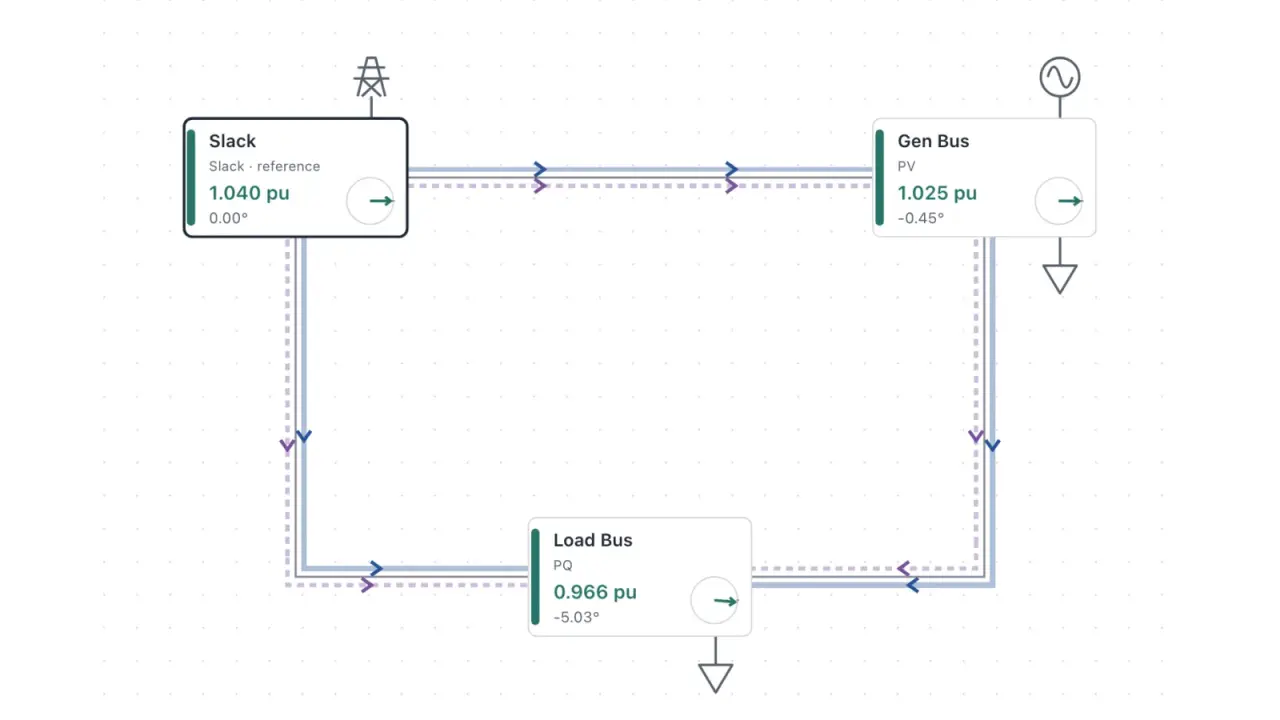
Solving AC Load Flow with Newton–Raphson in the Browser

Load flow, also called power flow, answers a steady-state question about an AC network: given what each generator is set to produce and what each load draws, what are the voltage magnitude and phase angle at every bus (a node where lines, generators, and loads connect), and how much power moves through each line?

The question is easy to state and hard to answer by hand. Each bus adds two nonlinear equations, each bus’s voltage depends on its neighbors’, and a realistic network has thousands of unknowns that have to be solved together. Changing one load can move voltages across the network in ways the equations do not make obvious. I built Load Flow Analysis, a browser tool that puts a network, its inputs, the solver, and the results on one page, so I can change an input and see the new voltages and flows on a diagram right away. Watching the network respond builds an intuition that working through the equations alone does not.

This post explains what load flow is and how Newton–Raphson solves it, then how the tool runs the solver in the browser.

The power flow equations

Line impedances form an admittance matrix $Y$ , and bus currents follow from bus voltages through $I = YV$ . If the inputs were currents, one linear solve would finish the job.

The inputs are powers. Complex power at bus $i$ is voltage times conjugate current, so the unknown voltages multiply each other:

\begin{aligned} S_i = P_i + jQ_i &= V_i I_i^* \\ &= V_i \sum_j Y_{ij}^* V_j^* \end{aligned}

Separating the real and reactive parts, with $Y_{ij} = G_{ij} + jB_{ij}$ and $\theta_{ij} = \theta_i - \theta_j$ , gives two real equations for every bus:

\begin{aligned} P_i &= \sum_j |V_i||V_j| \big( G_{ij}\cos\theta_{ij} \\ &\qquad\qquad + B_{ij}\sin\theta_{ij} \big) \\ Q_i &= \sum_j |V_i||V_j| \big( G_{ij}\sin\theta_{ij} \\ &\qquad\qquad - B_{ij}\cos\theta_{ij} \big) \end{aligned}

They multiply unknown magnitudes by sines and cosines of unknown angles, so they are nonlinear.

PQ, PV, and slack buses

Each bus has four quantities, $|V|$ , $\theta$ , $P$ , and $Q$ , and two equations. Two of the quantities have to be given, and which two depends on the equipment at the bus:

PQ (load) bus: $P$ and $Q$ are given, because a load is described by what it draws. The solve finds $|V|$ and $\theta$ .
PV (generator) bus: $P$ and $|V|$ are given, because a generator is set to a real power output and a voltage setpoint. The solve finds $\theta$ , and $Q$ is whatever it takes to hold that voltage.
Slack bus: $|V|$ and $\theta$ are given. $P$ and $Q$ come out of the solution.

The slack bus is there for two reasons. The equations contain only angle differences, so one bus has to define zero. And real power cannot be specified everywhere, because line losses are unknown until the voltages are known, so one source has to make up the difference.

The solve uses only the equations whose left side is known: $P$ at every PV and PQ bus, and $Q$ at every PQ bus. That leaves one unknown angle for every bus except the slack and one unknown magnitude for every PQ bus. Line flows follow directly from the voltages at each end once the solve is done.

Solving the equations with Newton–Raphson

Newton–Raphson is the usual way to solve these equations. The mismatch is the gap between each bus’s specified power and the power the equations give at the current guess:

\begin{aligned} \Delta P_i &= P_i^{\text{spec}} - P_i(\theta, |V|) \\ \Delta Q_i &= Q_i^{\text{spec}} - Q_i(\theta, |V|) \end{aligned}

The Jacobian $J$ holds the partial derivatives of $P$ and $Q$ :

J = \begin{bmatrix} \partial P/\partial\theta & \partial P/\partial|V| \\ \partial Q/\partial\theta & \partial Q/\partial|V| \end{bmatrix}

Each iteration solves this linear system, adds the result to the guess, and recalculates the mismatch and Jacobian at the new point:

J \begin{bmatrix} \Delta\theta \\ \Delta|V| \end{bmatrix} = \begin{bmatrix} \Delta P \\ \Delta Q \end{bmatrix}

The tool works in per unit, where 1 pu of voltage is nominal and 1 pu of power is 100 MVA in its reference cases. It begins from a flat start, with every unknown magnitude at 1 pu and every unknown angle at zero, and stops when the largest mismatch falls to $10^{-6}$ pu.

Client-side state and data flow

The LoadFlowWorkspace component keeps the network in a single editor state. Choosing one of the seven reference cases or an empty network replaces that state, and edits update it. Five of the cases are standard benchmark networks of 9 to 118 buses, adapted from MATPOWER.

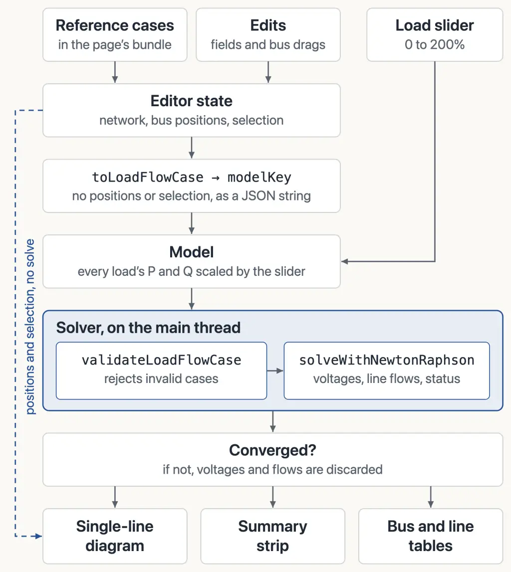
toLoadFlowCase copies the electrical model out of that state for the solver, without bus positions or the selection. The model is memoized on the JSON string of that copy, modelKey, and on the load slider’s value. The slider scales every load’s $P$ and $Q$ together and leaves generator $P$ setpoints fixed, so the slack bus supplies all of the added real power and the added losses.

The solver runs during render

The tool solves as the inputs change, without a Run button or a worker. runLoadFlow is called inside a useMemo, so a new model reruns it during render, on the main thread.

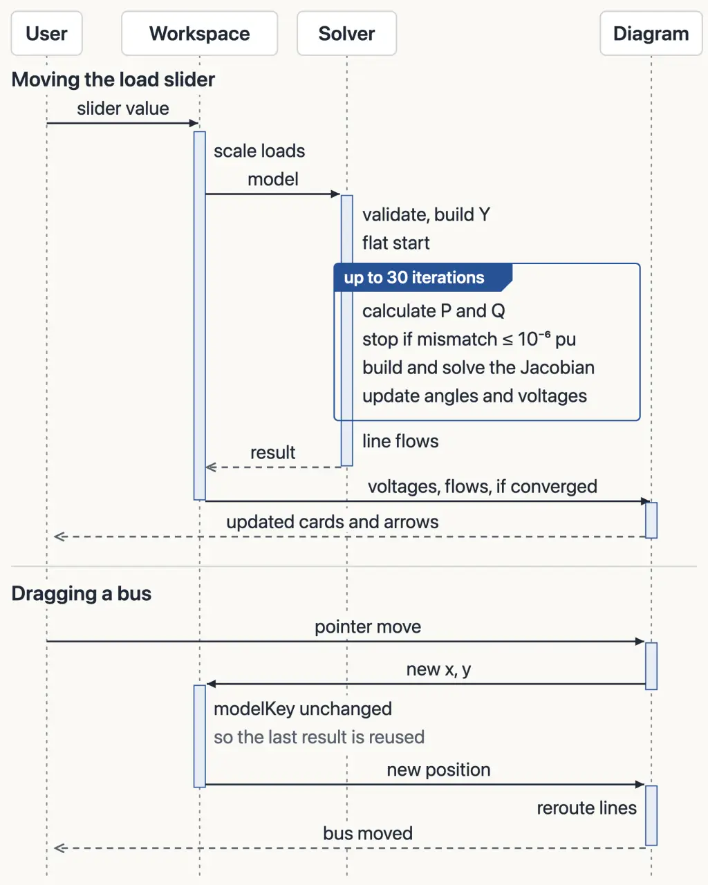
A slider step on the 118-bus case takes about 50 ms in Chromium on an Apple M4 when the solve converges. Dragging a bus takes the second path in the figure: its new position changes the editor state but not modelKey, so nothing is solved again.

Reading the single-line diagram

A single-line diagram draws each balanced three-phase circuit as one line. In the tool, each bus is a card showing its type, voltage magnitude, and angle relative to the slack bus. Its color shows a voltage band, a visual guide rather than an equipment limit. Real power is drawn in solid blue and reactive power in dashed purple, together or one at a time.

On the default three-bus network, dropping 30 MVAr at the Load Bus raises its voltage more than twice as much as dropping 30 MW. The equations say so, but the diagram makes it obvious.

Each line is drawn as two halves with separate arrows, because the power at its two ends can differ. The tool reports power as positive into the line at each end, following MATPOWER’s branch convention, and the sum of the two is what the line absorbs. In the IEEE 9-bus case below, the arrows on the Bus 2–Bus 8 branch meet in the middle, with reactive power entering from both ends.

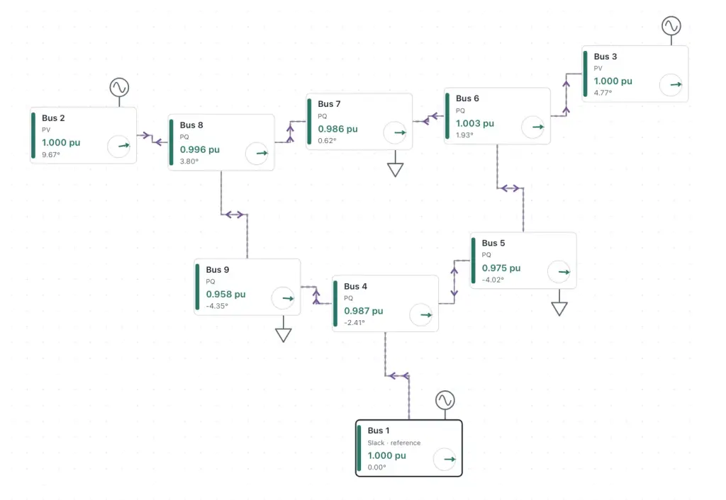
The tool’s IEEE 9-bus diagram in its reactive-power view, with bus cards showing voltages and angles and purple arrows meeting in the middle of the Bus 2–Bus 8 branch

The diagram, including dragging buses and arranging them automatically, was the harder part of building the tool for me.

Limits and future work

The network is not easy to edit. The diagram is for selecting and arranging, not editing. Parameters are edited one bus or line at a time in a form below it, and both that form and a separate panel for adding and connecting buses start collapsed. The form also has no field for shunt capacitors, though the solver models the ones in the IEEE cases. And the tool shows only the current solution, so seeing what an edit changed means noting the voltages beforehand. Editing on the diagram, with each bus shaded by how far its voltage moved from a saved solution, would let the diagram show both the edit and what it changed.

A PV bus’s $Q$ is whatever it takes to hold its voltage. The case data gives each generator reactive limits, but the solver does not enforce them, so under heavy load the tool can show healthy voltages that depend on generators exceeding theirs. In the IEEE 14-bus case at 150% load, it reports “Converged” with every bus at 1.00 pu or above, while all four PV generators are past their limits: the one at Bus 2 supplies 101 MVAr against a limit of 50. Holding those four at their limits and solving again, with the slack bus still unlimited, drops Bus 14 to 0.903 pu. “Converged” here means only that the power balance holds at every bus, not that generators stay within their limits or lines within their thermal ratings.

Scale is the last limit. Each bus connects to only a few others, so most of the Jacobian is zero. The solver still stores it as a dense matrix and solves it by Gaussian elimination. On the 118-bus case, this fits within the slider-step time above, but a network with 100 times as many unknowns would need about a million times the work per iteration. The tool’s cases are small next to the utility models I had seen in PSS/E. I did not try one that large in the browser, and with a dense solver I doubt it would run well.